Epidemiology

TYPES OF STUDIES

Cross-sectional studies: observational studies in which exposures and outcomes (e.g. a disease state) are measured simultaneously in a population. (Single time point, don’t know about temporal nature of exposure or outcome. CAUSALITY NOT IMPLIED)

Case-Control studies (retrospective): observational studies in which we identify a group with a particular outcome and another group without the outcome and compare their past exposures.

Prospective Cohort studies: observational studies in which we follow a population forward in time collecting data on exposures (subjects chosen based upon exposures) and the development of outcomes. MUST CHOOSE INDIVIDUALS WHO DON’T HAVE OUTCOME (CAUSALITY IMPLIED)

Randomized Controlled Trials (RCTs): experiments in which we randomly assign participants to a treatment group (the exposure) or a comparison (often a placebo) group and follow them forward in time for an outcome (CAUSALITY MORE STRONGLY IMPLIED)

TYPES OF VARIABLES

Independent Variable: A variable we measure or manipulate (as an intervention or treatment) that may be associated with an outcome of interest. If it occurs before development of an outcome, it is sometimes called an exposure or predictor variable.

Dependent Variable (Outcome): Measurable outcome of interest (e.g. a disease state, cure, or death) which we’d like to predict or explain with independent variables/predictors.

Nominal or Categorical: named but not necessarily ordered (may be dichotomous) – (e.g. sex, death, ethnic or cultural background).

Ordinal: necessarily ordered categories where the distance between each unit is not defined (e.g. military ranks; or, a satisfaction scale of poor, fair, good, very good, excellent)

Interval (Discrete): take on discrete (e.g. integer) values with equal magnitude between points (e.g. number of medications)

Interval (Continuous): may take on any value over a continuum (e.g. height or weight)

MEASURES OF FREQUENCY

Prevalence: How many people have an outcome at a given time point (people with outcome/total people analyzed). Ratio or percentage reported. CROSS SECTIONAL STUDIES WILL REPORT PREVALENCE.

Incidence: How many people develop a given outcome over a specified period of time. COHORT STUDIES AND RCTS CAN REPORT INCIDENCE

MEASURES OF ASSOCIATION

Absolute Risk: risk difference between groups (subtraction). Ex: If smokers have a 50% risk of getting lung cancer, and non smokers have a 5% risk, smokers have a 45% greater chance of getting lung cancer (when compared to non smokers).

Relative Risk: proportion with an outcome in one group divided by proportion with the outcome in another. (The details of the calculation vary by study design.)

The measure of “relative risk” in a cross-sectional study is actually a prevalence ratio =

[prevalence among those with an exposure (attribute)]/ [prevalence among those without an exposure (attribute) ]

PROPORTION VS. ODDS

Proportion: the number of times an event occurs divided by the total possible number of possible opportunities (risk/percentage)

Odds: the number of times an event occurs divided by the number of times it does not occur (the number of times more likely the event is to occur than to not occur)

*When comparing risk ratios vs. odds ratios, odds ratios are usually further from 1. Odds are also able to be modeled from 0 to infinity (instead of 0 to 1 like risk) allowing for logistical regression.

THREATS TO THE INTERNAL VALIDITY OF A STUDY

Chance: random error that makes differences appear significant/insignificant (depending on the scenario.

Bias: Systematic error introduced during design, subject selection, data collection, or analysis.

Confounding: Factors related to both predictor and outcome which obscure their true relationship (factors that correlate to the outcome, but are not causal).

Generalizability: To what populations outside of the study can the conclusions be applied (also called “External Validity”)

COHORT STUDIES MORE IN DEPTH

Cohort studies: “Natural Experiments” in which we follow a defined group of individuals:

Prospective cohort study: individuals enrolled then followed forward in time (best)

Retrospective cohort study: investigators go back in time to assemble the cohort or use data collected for non-research purposes. Outcomes may be continuous variables (e.g. systolic blood pressure) but are often categorical (disease onset, death, etc.).

Follow-up time may be fixed (all individuals followed for 5 years) or variable (each individual contributes some amount of person-time to the denominator). 

Cumulative incidence = # of new outcomes / total # persons at risk at the start of follow-up. (It is a unitless fraction, but the observation period is described (e.g. “the annual incidence of pancreatic cancer among men 40-50 years old”).

Incidence rate (incidence density) = # of new events/ sum of total person-time at risk (e.g. 20 cases per 1000 person-years). (Note: The denominator of an incidence rate is the sum of person-time contributed by each member of a population observed. For example, a person-year is one person followed for one year, or one person followed for 3 months together with another followed for 9 months, or 52 people each followed for a week, etc…)

**Cumulative incidence is usually used when all people are followed for an equal time period to see if they have an event, while incidence rate allows for different lengths of follow-up.

Risk for an individual: can be calculated as cumulative incidence or as incidence rate x time exposed

RELATIVE RISK VS. ODDS RATIOS

The 2 x 2 table is the standard representation of data with a dichotomous outcome. Outcomes are usually found in the columns, and exposures in the rows:

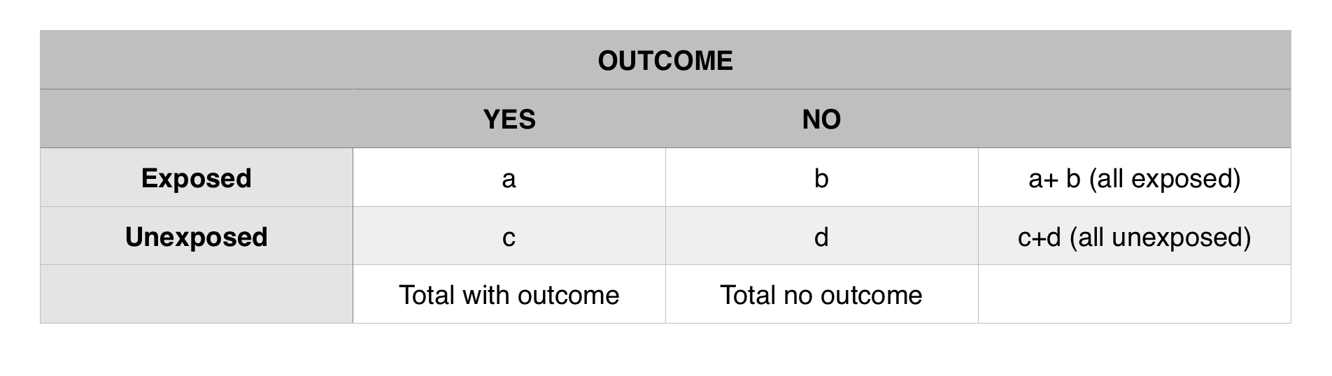
Below is the math used to calculate a relative risk (RR) vs. an odds ratio (OR) based upon the table above.

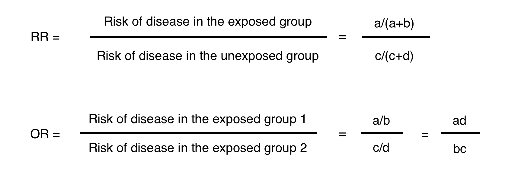
**Odds ratios are close approximations of risk ratios when the outcome is rare (a frequently used rule of thumb is <10%). When the outcome is more common and/or the association is stronger (RR further from 1.0) the OR will be a less good approximation of the RR. In these cases, the OR will be more extreme (higher than the RR if they are > 1.0 and lower than the RR if they are < 1.0). 

Attributable risk (AR) (or absolute risk difference): describes the increased risk of disease that is due to the exposure (among the exposed). Even in the exposed group, not all disease results from the exposure of interest; some disease is the result of other causes.

AR = Risk of disease in the exposed – Risk of disease in the unexposed = [a/(a+b)] – [c/(c+d)]

**The concept AR is made more complex than it needs to be. Here is a quick example of how simple it is. If there is a 50% chance a smoker will get lung cancer, and a 5% chance that a non smoker will get lung cancer, then the AR here (relative to smoking) is 45%. AR a measure of absolute risk difference that is attributed to a specific exposure.

Attributable fraction (AF may also be expressed as AR%) is the proportion of disease in the exposed group that is due to the exposure. The numerator in this calculation (below) is the AR.

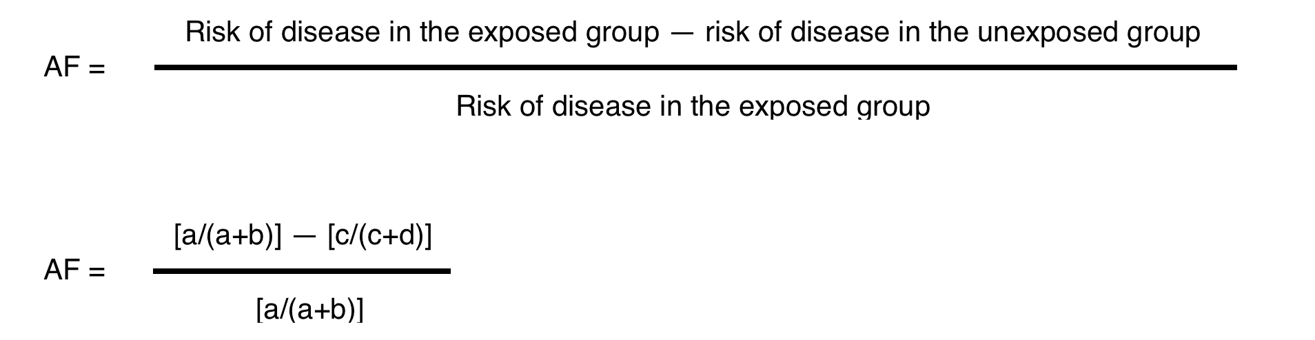
*The goal here is to find out what percentage of people in an exposed population can have their outcome attributed to an exposure. From the previous example, what fraction of smokers have will get lung cancer because they are smokers? Calculation is 45%/50% = 0.90 (90%). So in this example, 90% of lung cancer cases in smokers can be attributed to the exposure “smoking”.

**AR MEASURES AN ABSOLUTE RISK DIFFERENCE WHILE AF IS A PROPORTION

POPULATION ATTRIBUTABLE RISK/FRACTION 

Population Attributable Risk (PAR): incidence of a disease in a population associated with an exposure.

PAR= (AR)*(prevalence of exposure in a population)

**To continue the above example, if AR of smokers for lung cancer is 0.45 (45%) and half of the people in a population are smokers (0.50/50%) than the PAR is the product of these two values (PAR = 0.45*0.50 = 0.275). PAR is looking at the incidence of an outcome in a TOTAL population that is attributed to an exposure. 

Population Attributable Fraction (PAF): Proportion of disease in a population associated with an exposure.

PAF= PAR/Total Incidence of Disease in Population

**To continue the smoking example. Above PAR was calculated to be 0.275. If the total incidence in a population is 0.35 (total cases of lung cancer over total population analyzed) than PAF = 0.275/0.35 = 0.786. PAF is looking at the proportion of an outcome in a total population that is attributed to an exposure. 

SURVIVAL ANALYSES

Not all subjects in a cohort experience an outcome at the same time- and when they do often matters. Survival analysis examines the rate at which people reach the endpoint (or event) of interest. The “event” may be death, but could be infection, cancer remission, etc.

Attributes of survival analysis:

• Cohorts begin with 100% survival (or 100% event-free)
• The “number at risk” (denominator) changes over time (either because they experience the event or are lost to follow-up).
• Curves can be generated with points at pre-specified time intervals (life table analysis) or by plotting points at each time an event occurs (Kaplan Meier approach).
• Hazard ratios are used to describe the results from survival analyses, based on the ratio of events per person-year of observation time in exposed and unexposed groups – equivalent to incidence rate ratios.
• Statistical tests (e.g. log-rank test) can help assess whether 2 curves differ beyond what would be expected by chance.
  

Life-table(actuarial)method: standard increments of calendar-time (e.g. 3 months)

Kaplan-Meier method: time periods determined by each occurrence of an endpoint by a subject [most common]

For survival analysis “Number At Risk” remains in the denominator and this number is subject to change as study members get the outcome of interest, or are lost to followup. ONLY INDIVIDUALS WHO DO NOT GET THE OUTCOME AND REMAIN IN THE FOLLOWUP POPULATION STAY IN THE DENOMINATOR

HYPOTHESIS TESTING

Random Sample: a subset of the population we choose in which all individuals have the same probability of being chosen. Likelihood that a sample will be representative of the greater population is determined by its size and shape.

*We can reject the null hypothesis, but can not prove that it is true.

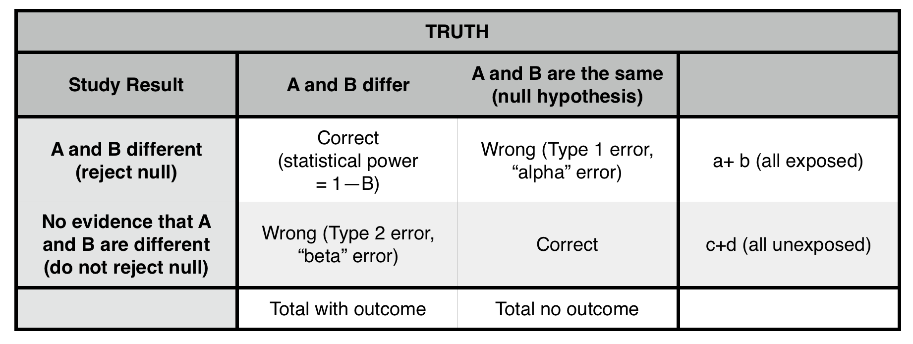
Type 1 error (α = probability of making a type 1 error):  concluding that two populations are different (rejecting the null hypothesis), when they, in fact, are not different (that is, they are drawn from the same population). The cutoff for α at 0.05 (the p-value) is generally taken (arbitrarily) as the risk of alpha error below which we are comfortable rejecting the null. ONLY POSSIBLE IN A POSITIVE STUDY (false positive). Lowering p value cutoff will decrease this error risk.

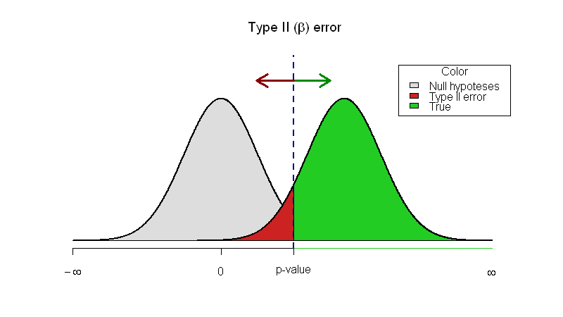
Type II error (β = probability of making a type II error): not concluding a difference exists (not rejecting the null), when the samples, in fact, are drawn from different populations. ONLY POSSIBLE IN A NEGATIVE STUDY (false negative). Sampling a larger population will likely decrease this risk.

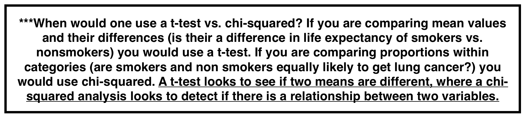
T-Test: a t-test compares two means. The null hypothesis is that both of these means belong to the same population.

T statistic (for 2 independent samples) is a comparison of the difference in the sample means compared to the expected variability in sample means. How likely is it that both of these means belong to the population given the expected mean variability? 

Two tailed t-test: tests differences between means in both directions (if mean is lower or higher in a statistically significant manner). Should be used MOST of the time.

One tailed t-test: tests differences in between means in one direction (less conservative).

Chi-squared test: Seeks to determine whether an association exists between two categorical variables. Analyzes a 2×2 table by comparing observed vs. expected if the null hypothesis were true (i.e. if the proportion of outcomes were equal in the two groups). Look up p value for test statistic from formula below. The lower value for chi squared the higher p value.

*Note: the “expected” value in any cell = (row total x column total) / total n of table. We use the total population to model our “expected” values.  

STATISTICAL SIGNIFICANCE

 P-value: probability that the result seen is due to chance (and not to a real difference in populations). Factors that impact p-value are:

• Magnitude of difference: larger differences are more significant.
• Size of sample: increasing sample size will lower the p value for a difference (even if the magnitude is unchanged).
• Spread of data: the less variable the data is the lower the p value will be for a given observed difference (even if magnitude is unchanged).

Important Caveats: P value thresholds are arbitrary, statistical significance does not equal clinical relevance, and bias is often times present so minimizing random chance (with a lower p value) isn’t the most pressing issue (with most studies).

CONFIDENCE INTERVALS

P value: a p value on its own provides the probability that an observed result is due to random chance (under the null hypothesis). However, P values provide no information on the results’ precision—that is, the degree to which they would vary if measured multiple times. 

Confidence Interval (CI): a confidence interval will give information on the precious of a result and the percentage of time the value should fall in a interval if the results were measured multiple times. Some ways to phrase what a CI means:

“95% of the time the true effect of the exposure will be within the range from X to Y”

“The interval computed from the sample data which, were the study repeated multiple times, would contain the true effect 95% of the time.”

Factors that influence CI: 

• Sample size: the larger the sample the narrower the CI will be.
• Variability in the data (standard deviation): the narrower the spread of the data the smaller  the CI will be
• Degree of confidence: the higher the confidence percentage (99% vs. 96% interval) the larger the CI will be

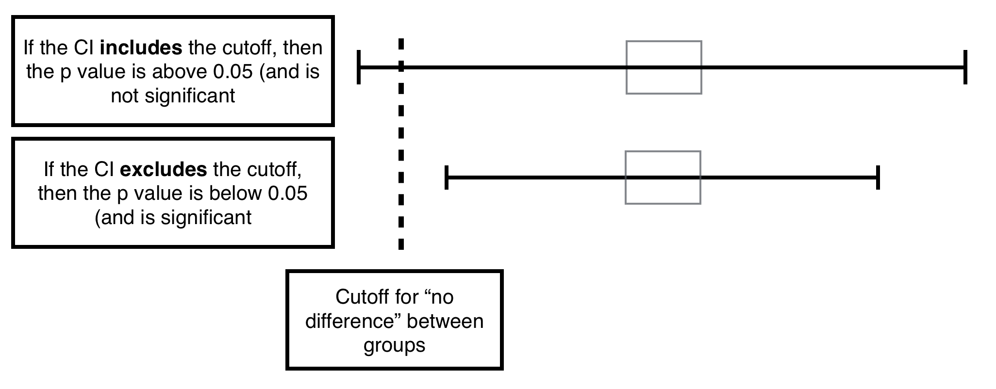
Relationship between CI and P value: if the cutoff for “no difference” is included in the CI likely the p value is not significant. If it is not included in the CI it likely is significant. If it borders the interval (exactly) likely the p value is exactly the min significant value. 

The 95% confidence interval around the mean of a normally distributed continuous variable is given by: Mean + 1.96 x SEM (not the SE of the total pooled population).

ROLE OF 95% CIs IN ASSESSING TYPE II ERRORS 

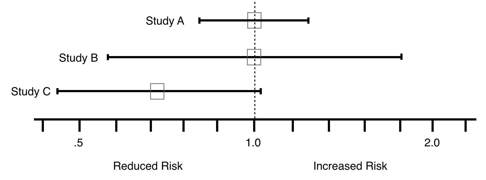
The best way to decide whether a type II error exists is to ask two questions: 1) Is the observed effect clinically important? and 2) To what extent does the confidence interval include clinically important effects? The more important the observed effect and the more the confidence interval includes important effects, the more likely that a type II error exists.

In line with this, looking at the examples below, if the goal was to reduce RR, Study C shows promise and should be repeated (Type 2 error chance here is much higher compared to study A and B).

*** IMPORTANT REALIZATION TO MAKE. The confidence interval utilizes the SE (standard error) of the specific mean (which the interval is being made for, n used for calculation only includes population for this mean). T statistics will be calculated using the SE of the pooled population (n used will include the total population)***

TYPES OF BIAS

Bias: Systematic departures from the true estimate of the risk of an exposure on the disease/outcome. Can occur in study design, data collection, and/or analysis. Can lead to over or underestimation of risk.

Selection Bias: most evident in case controlled study. Samples compared are chosen such that they represent different underlying populations than those we wanted to compare Selection bias makes your sample non representative of the source population. It has nothing to do with generalizability (application to other populations).

Information Bias (Ascertainment bias): Difference in accuracy or completeness of information in the study groups.

2 types Differential vs. non Differential Misclassification:

Differential bias: Recall bias (altered memory in a skewed fashion around an event), higher rates of screening between study groups leading to higher cancer rates in one group (cancer detection varies, not rate here).

Misclassification Error: Example: a lab test is only accurate a small percentage of the time, as a result you are likely to misclassify your control and treatment groups.

CONFOUNDING

Confounding: Distortion of the effect of one risk factor (exposure, predictor) by the presence of another. A confounding factor may mask an actual association or create the appearance of an association even if a true association is absent.

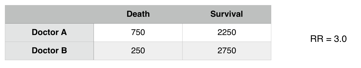
In the above example it seems as though Doctor A has worse patient outcomes (RR3.0 with respect to death) however when considering other factors, it seems as though there is a confounding variable here: patient status.

***THE RELATIONSHIP HERE WE ARE DRAWING IS BETWEEN DOCTOR A AND DEATH RATE IF PATIENT STATUS IS RESPONSIBLE FOR MORE DEATHS THIS IS A CONFOUNDER FOR THE UNDERLINED ASSOCIATION.

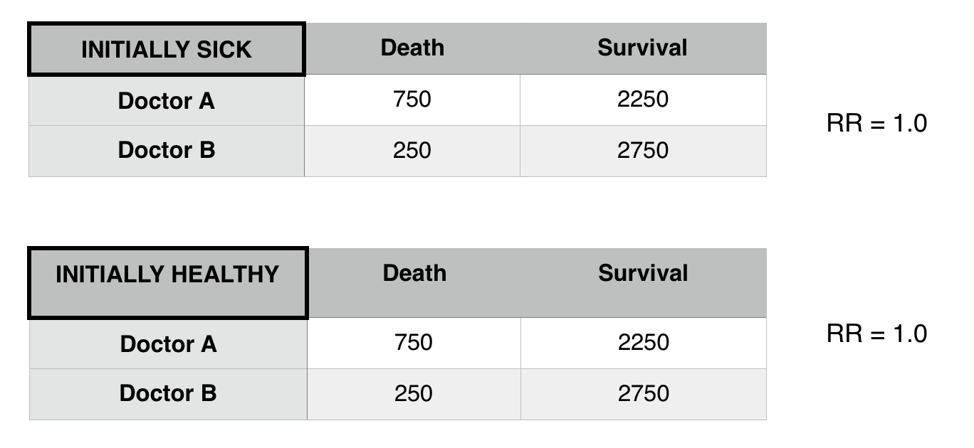
Now that we control for patient status we see that there is difference in death risk between doctors A and B. Patient status was confounding the relationship between Doctor A and B. 

Properties of Confounders: 

1. A confounder must be a cause (or be a risk factor for) the outcome.
2. The confounder must be related to the exposure, i.e., have a different value at each level of of the exposure. For cohort studies or randomized clinical trials, this condition must hold at baseline.
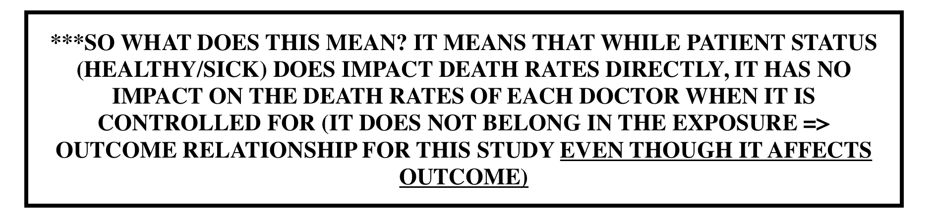
3. The confounder must NOT be on the causal pathway between the exposure and outcome (not an intermediate variable).

Preventing Confounding (During Study Design):

• Restriction: Only look within a population that either has/does not have the confounder (in above example, only analyze healthy patients).
• Matching: Compare the same amount of individuals who have/do not have the confounder between populations (analyze the same amount of healthy and ill patients for each doctor).
• Randomization: randomize individual that do and do not have the confounding variable (randomize patients that are healthy and ill to be treated by either doctor).

Preventing Confounding in Analysis Phase: 

Stratification

• Analyze in 2 (or more groups) that are homogeneous with respect to the potential confounder
• Effects in the strata will be equal to each other, but different from the effect if all subjects lumped together (crude effect)

**This was observed in the above example. 

EFFECT MODIFICATION 

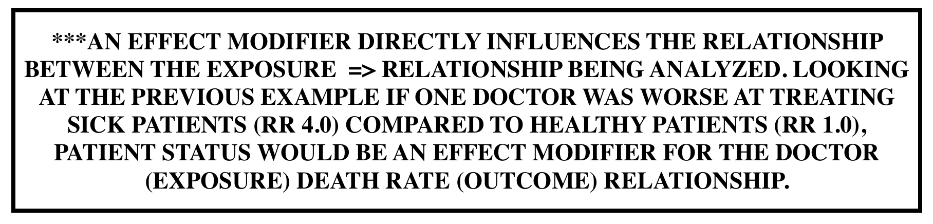
Effect modification vs. confounding: Unlike confounders, effect modifications are important to the exposure =>outcome relationship that is being tested. Effect modifiers reflect underlying biological differences in the mechanism of effect for levels of a 3rd variable.

• Differing ORs/RRs for each level of a 3rd variable
• It is a finding that is to be reported, not avoided

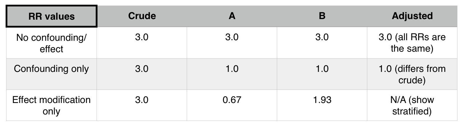
STRATIFIED RESULTS: 

If stratifying by a factor (such as patient status) does not change the stratified relative risks (when compared to the initial pooled relative risk) that factor is not a confounder or an effect mediator.

If If stratifying by a factor (such as patient status) does change the stratified relative risks (when compared to the initial pooled relative risk) AND each of these new stratified relative risks equal one another, that factor is a confounder.

If If stratifying by a factor (such as patient status) does change the stratified relative risks (when compared to the initial pooled relative risk) AND each of these new stratified relative risks equal one another, that factor is a effect mediator.

POWER

Alpha error value can be thought of as the p-value threshold we are using (e.g. 0.05). It is the probability of type 1 error.

Beta (ß error value is the probability of type 2 error).

Power is 1- ß. Chance you won’t make type 2 error. The chance that you will conclude, from your sample, that there is a difference between the groups (reject null) at the level of significance (alpha) that you have pre- specified (PROVIDED A DIFFERENCE REALLY EXISTS).

*lowering p-value increases alpha error, decreases ß error, and increases power.

**Increasing sample size and decreasing variability both also decrease ß error (increasing power).

What increases the power of a study?

• Increasing the size of the sample
• Increasing magnitude of desired detectable difference (the larger change you are looking for, the easier it is to detect)
• Increasing alpha error
• decreasing standard deviation (the smaller standard deviation the more power).

SCREENING

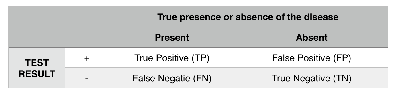
Sensitivity: how often is the test able to correctly identify the presence of a disease in those who have the disease? TP/ (TP+FN)

Specificity: how often does the test correctly identify the absence of a disease in those who are disease free? TN/(TN+FP)

Positive predictive value: post test probability of having a disease given a positive test result. TP/(TP+FP)

Negative predictive value: post test probability of not having a disease given a negative result. TN/(TN+FN)

*A perfectly sensitive test: is one that never misses disease (no false negatives).

*A perfectly specific test: is one that never indicates disease when not present (no false positives).

CRITERIA FOR CAUSALITY 

Sir Bradford Hill’s Criteria of Causality

1. Strength of association
2. Specificity
3. Temporality
4. Reversibility
5. Analogy
6. Plausibility (based on known mechanisms, consideration of alternative explanations)
7. Dose-response relationship (biologic gradient)
8. Consistency (across studies)

Equipoise: a state of uncertainty about the direction the study results would go in. Equipoise is the central ethical criterion required to enroll patients in a randomized trial.